Introduction
Whenever someone measures a physical quantity--for example, a
length measured by putting a ruler beside it or a mass measured
by comparing it with known masses on a balancethere
is some range of uncertainty in the result. No quantity is ever
measured with complete precision. In the examples cited, one
can imagine some reasons for the uncertainty. Limitations of
eyesight make it impossible to tell precisely where the end of
the object falls on the ruler. If the length is read to be 10.25
cm, it could actually be l0.255 cm or 10.245 cm and look exactly
the same to the eye. Similarly, there will be a range within
which mass may be added or subtracted from the balance pan without
upsetting the appearance of balance. Such effects will lead with
equal probability to measurements that are too high or too low,
and a single observer will probably get different values within
the range of uncertainty for successive measurements. Errors
of this sort are referred to as random. There may also be sources
of systematic error which lead consistently to a number which
is too large or too small. This could happen, for instance, with
a wooden ruler which had absorbed water on a humid day and increased
its length or with a balance which had not been properly balanced
when both pans were empty. Systematic errors are more difficult
to detect than random errors because they do not produce different
values for successive measurements. Nevertheless, the validity
and usefulness of an experiment depends critically on the proper
assessment of systematic errors.
Probability Distribution
The uncertainty associated with random error may be estimated
by making a measurement several times and considering the distribution
of results. It is often convenient to display the distribution
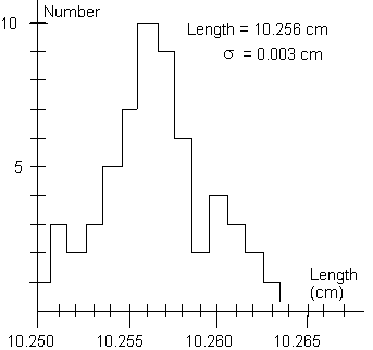
graphically as in Figure 1, where we have plotted on the horizontal
axis the measured value of a length and on the vertical axis the
number of times a particular value, or range of values within
a given bin, was measured. This type of graph is called a histogram.

| Length (cm) | Number of Times Measured |
| 10.250 | 1 |
| 10.251 | 3 |
| 10.252 | 2 |
| 10.253 | 3 |
| 10.254 | 5 |
| 10.255 | 7 |
| 10.256 | 10 |
| 10.257 | 9 |
| 10.258 | 6 |
| 10.259 | 2 |
| 10.260 | 4 |
| 10.261 | 3 |
| 10.262 | 2 |
| 10.263 | 1 |
Figure 1
Figure 1 illustrates a common property of such a series of measurements.
The values usually tend to cluster around a central value, in
this case around 10.256 cm, showing a "peak" of high
probability for measuring values close to the center and showing
fairly symmetrical "tails" of low probability for values
far from the center.
Given the data shown in Figure l, what can we conclude about the true value of the length being measured? Can we say only that the length is somewhere between 10.250 cm and 10.263 cm? While it is probable that the true value lies somewhere within this range, it is most likely that it is somewhere near the center of the distribution. Our best guess for the true value will be the average (or mean) of the distribution, which is defined as
 ,
,
where  is the number of times the value
 occurs and where N is the total
number of measurements,
The most common way of assigning a size to the uncertainty associated
with random error in a single measurement is to calculate the
standard deviation  of the distribution
from the formula
 ,
,
or equivalently
 .
.
The standard deviation is a measure of the uncertainty associated
with a single measurement. A typical measurement can be expected
to be about a standard deviation away from the mean value. Of
course, some measurements have a smaller difference from the mean
than  and some have a larger difference.
Sometimes one uses the relative error (
 ,
written as a percentage) to express the uncertainty in a single
measurement. For the data of Figure 1,
  =
l0.256 cm,
  = 0.003 cm, and
  /
/ = 0.0003 = .03%. Having guessed that, of all the estimates discussed,
the mean value of the distribution of measurements is closest
to the true value of the quantity, we can ask "How much confidence
should we have in this guess?" The answer is given by statistical
theory: the average difference of the mean from the true value
is of a size
  given by
 .
.
This number  is often called the standard
deviation of the mean, but it is important to distinguish
it from the standard deviation
  of a single
measurement. If we were to take more measurements (i.e., increase
N),
  should not change much, but
 would become smaller. We often use this
quantity
  as an error figure to accompany
a measured number, so that x = 5.7 ± 0.2 cm means that the
best estimate is
  = 5.7 cm and the uncertainty
associated with this estimate is
  = 0.2
cm.
Normal Distribution
According to statistical theory, a measured probability distribution
such as Figure 1 can be approximated by a "normal distribution
function"

where  is the number of measurements between
x and x + x and where N is the total
number of measurements.
  and
and  are the mean and the standard deviation. The notation "exp[...]"
means raise the quantity
  to the power
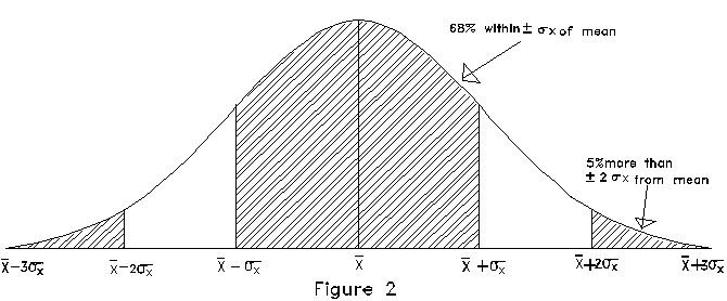
given in the square brackets. The normal distribution function
is plotted in Figure 2.

Note again that there are long tails, indicating that a small
fraction of the measurements will be much more than  away from the mean value. For the normal distribution, 5% of
the measurements will be more than ±2
 away
from
  while 68% are within
  of
of  . This well-known distribution is
also sometimes called the "Gaussian" distribution or
the "Bell-curve."
Subjectively Estimated Errors
Sometimes it is not practical to make the large number of measurements
needed to calculate accurate estimates of the mean and standard
deviation; instead, just one measurement is available to use as
the estimate of the true value. In this case you must use your
judgment to estimate the uncertainty in this measurement. Several
factors may enter into this, some of which could be the following:
1) The uncertainty may come from how accurately you feel you can
read a measuring device. For example, the accuracy with which
you could read a ruler would depend on how closely spaced its
tick marks are, and on how steadily it could be held while the
measurement was being made.
2) There may be fluctuations in the conditions under which an
experiment was done which could affect the outcome of the experiment
but which were beyond the control of the observer. These might
include variations in temperature or line voltage.
3) Your model of the physical situation may be somewhat unrealistic,
so that no matter how precisely measurements are made, calculations
using these measurements will not give an accurate result because
the formulas aren't a totally accurate model of reality. An example
of this would be a calculation of the range of a projectile using
a formula that neglects air resistance: the result might be fairly
accurate for a bullet but not for a wad of paper, no matter how
precisely you measure its initial velocity.
You must take the various factors into consideration and then
exercise your best judgment in estimating the range within which
you are confident that the measurement lies. The hope is that
for random errors the estimate of the uncertainty that you make
this way would be comparable to the value of  you would obtain if you made the measurement several times.
Propagation of Errors
Once the uncertainty in a measured quantity x has been
found, it is often necessary to calculate the consequential uncertainty
in some other quantity which depends on x. Consider a function
f which depends on x and/or y:  .
.
A series of measurements of x and/or y will yield
 . We will assume that the best estimate
of f is
  or
or  .
(But note that
  defined this way is not
always the same as the mean of f obtained from the individual
value
  .)
.)
Examples of the way to find  , the standard
deviation of f, are given below:
(a) 


(The standard deviation for f is obtained by adding the
standard deviations for x and y "in quadrature.")
(b) 


(c) 


(The relative error for f is obtained by adding the relative errors for x and y "in quadrature")
(d) 


(e) 


where A and b are preciselyknown constants and b is positive.
(The relative error for f is b times the relative
error for x.)
The rules for calculating  need some explanation.
Let df be the small change in f which results
from small changes dx, dy in the quantities x, y.
One can then make the identifications:
  .
For example, let
  . Then,

With the above identifications, we obtain ( )
= n(
 ). As another example, let
 . Then
  . We
might conclude that
  . However, during
half of the time, the deviations in x and y will
be in opposite directions (as long as x and y are
measured independently) so that one expects
  to be less than
  . A careful statistical
analysis shows that
  should be added "in
quadrature." All the rules (a) through (e) can easily be
obtained by identifying differentials with standard deviations
and by replacing addition or subtraction by addition "in
quadrature."
PART I SHOULD BE COMPLETED BEFORE COMING TO THE LAB.
A. Consider a solid metal ball of mass M and diameter D.
You are given the problem
of determining the density of the metal by measuring M
and D.
density = 
The ball's mass is measured with a simple laboratory balance,
and the following results are obtained for M:
927 gm 929 gm 925 gm 927 gm 928 gm
929 gm 930 gm 928 gm 929 gm 927 gm
The ball's diameter is measured with a vernier caliper, and the
following results are obtained for D:
5.88 cm 5.83 cm 5.83 cm 5.85 cm 5.83 cm
5.81 cm 5.82 cm 5.84 cm 5.83 cm 5.82 cm
(a) Plot a histogram of the distribution of the ten values for
M, and find the mean value and the standard deviation of
the distribution.
(b) Do the same for the distribution of D values.
(c) Determine the density of the metal, and indicate the uncertainty
in your value.
B. Estimate the density of your own body. Do this by first estimating
the volume of your body, thinking of it as an assemblage of cylinders,
spheres, truncated cones, etc., and make the measurements necessary
to estimate the volume of each part. Note that the volume of
a truncated cone,

is  .
.
Your estimate of the uncertainty of the volume will not be determined
by calculating a standard deviation, since you need to make each
measurement only once, but rather by estimating the accuracy of
each measurement and of the model. Divide your total volume into
your mass (an object that weighs 2.2 lbs. on earth has a mass
of 1 kg.) to obtain an estimate of your density. Compare this
with the density of water. Do you float or sink in fresh water?

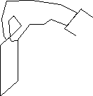
A. Measure your reaction time by trying the following: smooth
out a dollar bill and have a friend hold it vertically as shown.
Put your thumb and index finger on either side of the bill without
touching it, about halfway down for the first trial. When your
friend releases the bill try to catch it. (Do you see the makings
of a good bet here?) On subsequent trials, find out how far down
the bill you have to place your fingers in order to catch it,
and estimate the uncertainty in this. Use  to calculate an estimate of your reaction time, and calculate
the uncertainty in this estimate.
B. Now measure your reaction time by using a digital electronic
timer in "sensed start/stop" mode. In this mode, the
timer starts when one light beam is interrupted and stops when
the other light beam is interrupted. See how soon after someone
starts the timer that you can stop it. Repeat the measurement
a few times. Is the result of these measurements consistent with
the estimate of your reaction time and its uncertainty made using
the dollar bill?
As a way of generating data with a spread about a central value,
throw darts at the target (aiming for the central square) and
record the number of hits within each square. Throw at least 100
darts, more if you have the patience. (The target is on the last
page of this experiment.)
Add up the total number of hits on each row of the target. Find
the mean vertical position  and the standard
deviation
  . Make a histogram of the y
distribution and include on the graph a normal distribution curve
which has the same values of
  and
and  .
How well does this curve match your experimental distribution?
Is your value of
  at the center, within
the expected uncertainty? (If it is not, does this mean that you
are not aiming right?)
Now add up the total number of hits on each column of the target,
and repeat the previous exercise for the x distribution.
You now have your accuracy in the vertical and horizontal directions
(by the numbers  ). Why should you expect
these two numbers to be, or not to be, the same?
Geiger counters are provided to detect particles emitted from
radioactively decaying nuclei. A given nucleus decays at a random
time which cannot be predicted in advance. Thus, the distribution
of decays from a radioactive source will show statistical fluctuations
in time.
Measure the number of decays D registered by the Geiger
counter in a 15second time interval. Make this measurement
a total of twenty times. Calculate  from
your twenty values for D.
Statistical theory predicts that  for
this sort of random event (characterized here by the fact that
the probability that any one nucleus decays in a given time interval
is very small this sort of probability distribution is
called a Poisson distribution). Do your results approximately
agree with this?
