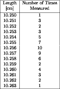
Table 1.1: Measured length of object.
The uncertainty associated with random error may be estimated by making a measurement several times and considering the distribution of results. Table 1.1 lists the results of a series of measurements of the length of an object.

Table 1.1: Measured length of object.
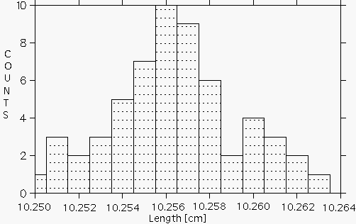
It is often convenient to display the distribution graphically as in Figure 1.1, where we have plotted on the horizontal axis the measured value of a length and on the vertical axis the number of times a particular value, or range of values within a given ``bin", was measured. This type of graph is called a histogram.

Figure:
Histogram of measured lengths.
Figure 1.1 illustrates a common property of such a series of measurements. The values usually tend to cluster around a central value, in this case around 10.256 cm, showing a ``peak" of high probability for measuring values close to the center and showing fairly symmetrical ``tails" of low probability for values far from the center.
Given the data shown in Fig. 1.1, what can we conclude about the true value of the length being measured? Can we say only that the length is somewhere between 10.250 cm and 10.263 cm? While it is probable that the true value lies somewhere within this range, it is most likely that it is somewhere near the center of the distribution. Our best guess for the true value will be the average (or mean) of the distribution, which is defined as
![]()
where
![]() is the number of times the value
is the number of times the value
![]() occurs and where N is the total number of measurements,
occurs and where N is the total number of measurements,
![]() .
.
The most common way of assigning a size to the uncertainty associated with
random error in a single measurement is to calculate the standard
deviation
![]() of the distribution from the formula
of the distribution from the formula
![]()
or equivalently,
![]()
The standard deviation is a measure of the uncertainty associated with a
single measurement. A typical measurement can be expected to be within
about a standard
deviation from the mean value. Of course, some measurements have a smaller
difference from
the mean than ![]() and some have a larger difference. Sometimes one
uses the relative error
(
and some have a larger difference. Sometimes one
uses the relative error
( ![]() , written as a percentage)
to express the uncertainty in a single measurement.
For the data in Table 1.1,
, written as a percentage)
to express the uncertainty in a single measurement.
For the data in Table 1.1,
![]() cm,
cm, ![]() cm, and
cm, and
![]() %.
Having estimated that, of all the estimates discussed,
the mean value of the distribution is closest to
the true value of the quantity, we can ask
``How much confidence should we have in this estimate?''
The answer is given by statistical theory:
the average difference of the mean from the true value is of a size
%.
Having estimated that, of all the estimates discussed,
the mean value of the distribution is closest to
the true value of the quantity, we can ask
``How much confidence should we have in this estimate?''
The answer is given by statistical theory:
the average difference of the mean from the true value is of a size
![]() given by
given by
![]()
The number ![]() is often called the standard deviation of the
mean, but it is important to distinguish it from the standard deviation
is often called the standard deviation of the
mean, but it is important to distinguish it from the standard deviation
![]() of a single measurement. If we were to take more measurements
(i.e. increase N),
of a single measurement. If we were to take more measurements
(i.e. increase N), ![]() should not change much, but
should not change much, but
![]() would become smaller. We often use this quantity
would become smaller. We often use this quantity
![]() as an error estimate to accompany a measured number, so
that
as an error estimate to accompany a measured number, so
that ![]() cm means that the best estimate is
cm means that the best estimate is
![]() cm and the uncertainty associated with this estimate is
cm and the uncertainty associated with this estimate is
![]() cm.
cm.